We, in the energy industry, have long used engineering calculations, aided by simple linear regression models, to estimate the energy saving potential of proposed interventions. However, as data sensors become increasingly ubiquitous and data storage costs continue to decline year over year, a shift away from this engineering calculation-based approach to a more data-centric approach is underway. For practitioners of energy efficiency, like us, this means a renewed focus on statistics and data management to enable a better understanding of the risks inherent in this data-heavy method of energy savings estimation.
What is linear regression and why do we use it?
When evaluating the energy saving potential of building retrofits or design, we use linear regression to estimate the dependence of one variable (dependent variable), such as energy consumption, on one or more independent variables such as ambient temperature. The goal is to determine the relationship existing between them. Establishing a linear relationship between variables allows us to predict future energy use, and therefore estimate future potential energy savings from a project with some degree of accuracy.
Assumptions of linear regression
Linear regression makes several assumptions about the data at hand. In the past, verifying the validity of these assumptions was not seen as an absolute requirement as the estimation methodology depended primarily on engineering wisdom established over decades. However, as the industry moves from being a discipline rooted in experience to one based on empirical and fact-based methods, the need for understanding these assumptions and their implications is higher than ever.
Four main assumptions of linear regression are:
- Linearity of data: The relationship between the predictor and the predicted is assumed to be linear
- Normality of residuals: The residuals are assumed to be normally distributed. Residuals are the difference between the predictor and predicted values.
- Homoscedasticity: (homogeneity of residual variance): The residuals are assumed to have a constant variance.
- Independence of residuals: The residuals are assumed to be independent of each other.
It is important to note here that time series datasets, such as those used in the energy industry, require significant transformations in order to satisfy all these assumptions. , so we will focus on finding the conditions under which deviation from these assumptions is minimal.
Let’s compare annual hourly and daily datasets of a facility to see how the above listed assumptions hold up. Each dataset contains four variables: time, energy, temperature, and energy predicted. The predictions for these datasets were created using a Time-of-Week and Temperature model based on Lawrence Berkeley National Laboratory’s paper, Quantifying Changes in Building Electricity Use, with Application to Demand Response.
Linearity of data
Linearity of data is checked by plotting the predicted values (predicted energy use) against the predictor values (time, energy, temperature). This method is straightforward when we have only one predictor variable; however, it gets increasingly tedious as the number of predictor variables increase. Another method to check for linearity in data is to plot the residuals against the predicted values.
The data fulfills this linearity assumption if the residuals are scatted randomly around the zero line.

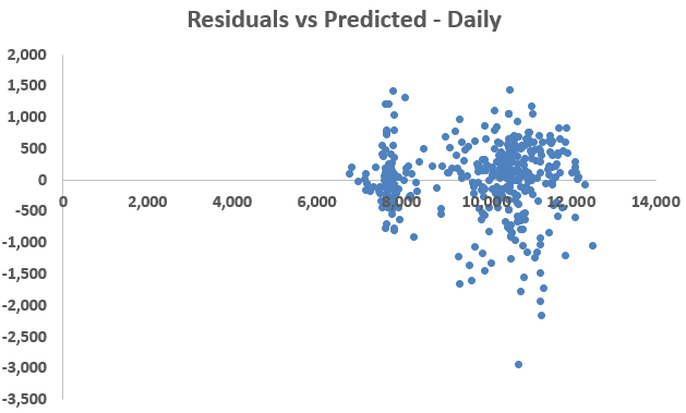
Figure 1: Residuals vs Predicted
A brief glance at Figure 1 shows greater amount of data above the zero line and greater deviations from the zero line on the bottom half of the graphs.
Normality of residuals
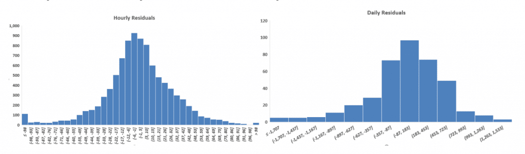
Normality of residuals is tested by plotting their histograms. Figure 2 shows that both the hourly as well as daily residuals are normally distributed.
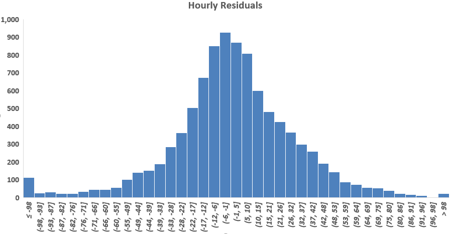
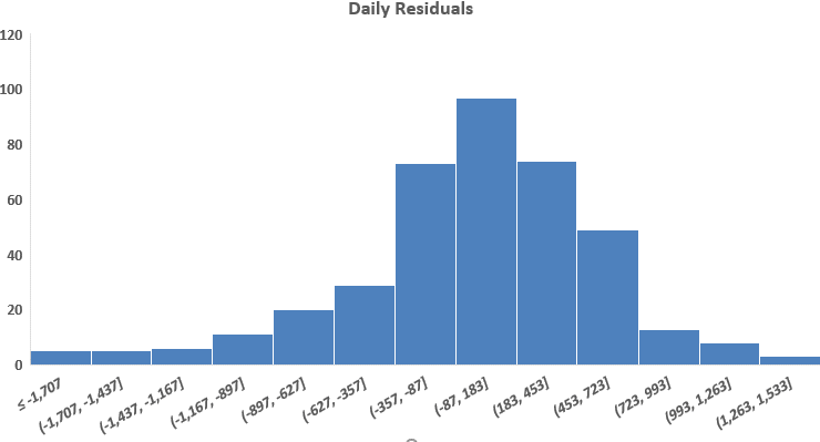
Figure 2: Residuals’ Histograms
Homoscedasticity
Homoscedasticity, or homogenous variance of residuals, is tested by plotting the residuals over time. Ideally, we would like to see a constant amount of scatter around the zero line. If the scatter increases or decreases over time, the dataset is in violation of this linearity assumption.
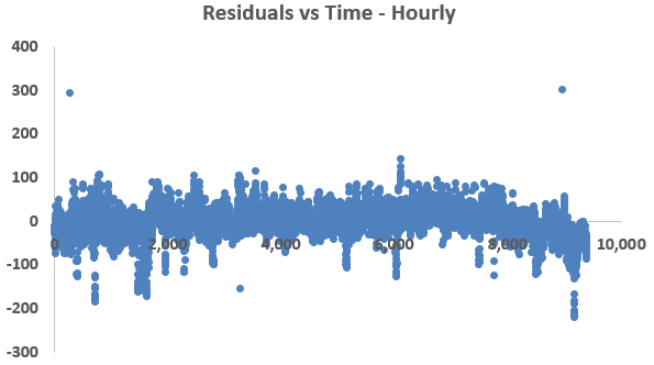
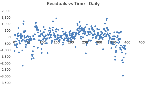
Figure 3: Residuals vs Time Observations
Figure 3 shows that the residuals, of both the hourly and daily models, have approximate constant variance except for the last few observations.
Independence of Residuals
When the residuals from different time periods (usually adjacent) are correlated, we say that the residuals are autocorrelated. It occurs in time series data when the errors (residuals) associated with one time period carry over into future time periods. While this does not affect the unbiasedness of the ordinary least-squares (OLS) estimators, it causes their associated standard errors to be smaller than the true standard errors, leading to the conclusion that the estimates are more precise than they really are.
We check for autocorrelation by plotting the errors against themselves lagged by one time unit in a scatterplot. The correlation coefficient of the residuals is calculated by taking the square-root of the coefficient of determination (R2).

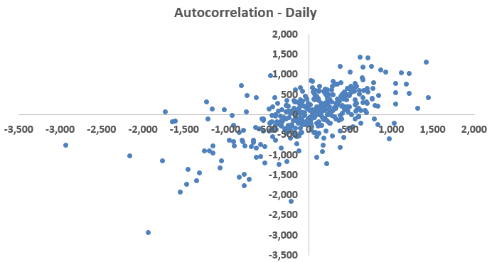
Figure 4: Autocorrelation
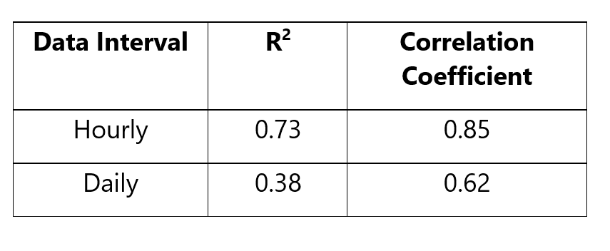
Table‑1: Correlation Coefficients
The actual residuals are plotted on the x-axis, and the residuals lagged by one time unit (the residual immediately succeeding the one plotted on the x-axis) are plotted on the y-axis of Figure 4. It shows that as a residual’s value increases (or decreases), the value of its immediate successor also increases (or decreases), implying a serial correlation, i.e. autocorrelation. R2, and its square-rooted value, are a quantification of this serial correlation. A higher value the correlation coefficient is indicative of a high linear relationship and high correlation between the x and the y variables.
It is clear from Figure 4 and Table 1 that both the hourly as well as the daily residuals are heavily autocorrelated. However, between the two the daily dataset has lesser correlated residuals.
Bringing it all together
Without transformation, time series datasets rarely satisfy all linearity assumptions. By comparison of the two datasets on each count, we conclude that the daily data violates the linearity assumptions to a lesser degree than the hourly data, and should, therefore, be used as the basis of empirical energy modeling for this facility.
There might be scenarios wherein a granular profile of operation is required for project implementation. For example, demand side management requires an understanding of hourly demand data. In cases like these, while a daily model might provide a more mathematically sound estimation, the hourly model will serve the purpose of visualizing and quantifying hourly demand better. Both hourly as well as daily modeling practices come with their own specific advantages and risks. As a practitioner, it will be up to you to balance the advantages against the risks to determine a data frequency that is most suitable for your purposes.
The linearity assumptions, along with the model’s prediction errors (CVRMSE), should be used to a build a comprehensive understanding of the modeling algorithm, its validity, and its applicability to energy efficiency projects. Just like you wouldn’t invest in an S&P fund if it didn’t track the S&P 500 index accurately, you shouldn’t use an energy model if doesn’t predict the facility’s energy consumption accurately. If you’d like to dive deep into your energy use data and need help identifying opportunities for energy savings, contact us any time.
Like this post? Share it with your network on LinkedIn.